In the following, we describe how each figure of the chapter 9 was obtained, in the hope that this will clarify the results presented and provide starting points for further simulations. Parts of these figures are also shown.
Figure 1 is a simple drawing.
Figure 2 was obtained from the theoretical formulas calling the fithifref and fithlifref M-files as follows
fithlifref(10, 0.5, 50, 2, [0:0.01:2.5])
fithifref(10, 0.5, 2, [0:0.01:2.5])
fithifref(10, 0.5, 0, [0:0.01:2.5])
Figure 3 was obtained by simulation of a Poisson spike train generator (n_th = 1, see the illustration below), an integrator with random threshold (n_th = 2, 5 and 10) and a perfect integrator model (time step 0.1 ms, 10 mV threshold, 0.5 nF capacitance, 2 ms ref. period). The ISI distributions are the theoretical ones, obtained using the gfitheor M-file.

Figure 4 was obtained by simulating an integrate-and-fire neuron for 1000 ms (time step 0.1 ms). The input was a Poisson pulse generator. The size of the pulses, capacitance and threshold of the model were adjusted to obtain a spike every 5th input.
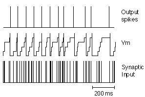
Figure 5 was obtained by a straightforward use of the theoretical formula given in the main text.
Figure 6 was obtained by simulating the model of tutorial 5 for 500 ms (time step 0.125 ms). The ISI distribution was obtained from the spike train spk_50 as explained in tutorial 5.
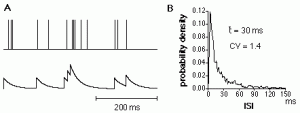
Figure 7 A was obtained as explained in tutorial 5 in the subwindow entitled NTA and Poisson spike counts. B was obtained directly from the theoretical formulas given by Cox (1962), see chapter 9 in ”Methods in Neuronal Modeling” for the exact reference (measuring interval = 200 ms, mean firing rate = 50 Hz).
Figure 8 was obtained by using the theoretical M-file prefdisp and the formula for the dispersion relation for a gamma distribution of order 2 given in sect. 4 of chapter 9 in “Methods in Neuronal Modeling”. The variance to mean relation for the retinal ganglion cell model was obtained by simulating the model of Tutorial 5 (the corresponding spike train is the one named spk_50 in the tutorial).
Figure 9 was obtained by using the M-file poissoncnt and roc (mean rates 40 and 50 Hz, counting time 200 ms). The likelihood ratio was obtained directly from the theoretical formula given in chapter 9 of “Methods in Neuronal Modelling”.
Figure 10. A:The roc curves were obtained using poissoncnt and roc with mean rates of 40 and 50 Hz and counting times of 200, 500, 1000 and 2000 ms. B: The ROC curve for the gamma distribution was obtained from the theoretical spike count distribution given by Cox (1962) (see chapter 9 in “Methods in Neuronal Modeling” for the exact reference) with mean spike counts of 8 and 10 spikes respectively and the roc M-file. The ROC curve for the Neyman type A distribution was obtained by calling the neymtacnt M-file (parameters: 8, 1.45, 25 and 10, 1.45, 25, in the two cases) and the roc M-file. The multiplication parameter 1.45 was taken to be identical to the one obtained at low firing rates in Tutorial 5.
Figure 11. The 3 Gaussian ROC curves were obtained by calling the gaussroc M-file. Transformation to normal coordinates was obtained in Matlab using the gamma function of Matlab (see Matlab reference guide).
Figure 12. The spike trains were obtained from a single long simulation (10 times10 sec, time step 0.5 ms) of the following model. Only the first 5 sec of each 10 sec stretch were used. Means were computed directly from the raw data using the Matlab sum function.
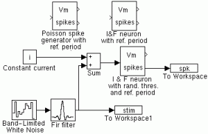
Figure 13. A: The functions m_x and rho for the renewal process of gamma order 2 were obtained directly form the formulas given in chapter 9 of “Methods in Neuronal Modeling”. B:The autocorrelation function of the gamma of order 10 process was obrtained directly form the gpstheor M-file (parameters: C=0.5 nF, V_thres = 10 mV, I = 0.4 nA, t_ref = 0, n =10, npoints = 1024, tstep = 0.5 ms). The delta peak at zero was subtracted.
Figure 14. Both power spectra were obtained from gpstheor (parameters: C = 0.5 nF, V_thres = 10 mV, I = 0.4 nA, n = 2/10, t_ref = 0, npoints = 1024, tstep = 0.5 ms).
Figure 15 was obtained by using the same model used in Fig. 12, the same stimulus s_0(t) was used for each simulation (10 simulation which lasted 10 sec for A and for B with different models, see above for the illustration of the models and below for a partial illustration of part A of the figure) and 1 sec of spike data was taken after 8 sec of simulation. Mean firing rates were computed in 50 ms bins using the Matlab sum function.
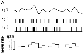
Figure 16. The power spectrum and LGN transfer functions were computed directly from the formulas given by Dong and Atick (1995, see sect. 6.3, chapter 9 in “Methods in Neuronal Modeling” for detailed references) and were plotted in double logarithmic coordinates. The spectrum of the output was obtained by simple multiplication and plotted in double logarithmic coordinates.
Figure 17. The theoretical transfer function (solid line in the illustration below) was obtained using the lgnfilt M-file. The method used to recover by cross-correlation the transfer function (dashed line in the illustration below) is described in details in tutorial 4 and sect. 7.1 of chapter 9 in “Methods in Neuronal Modeling” (the model is illustrated in the figure of sect. 4 above).
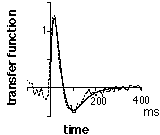
Figure 18. The data was generated using the same model as illustrated for fig. 12 (time step 0.5 ms, simulation time: 135000 ms). Simulation results were analyzed using the stimest (see A below) and psautostim (for the power spectrum shown in the inset to part B below) M-files.
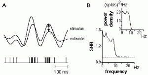
Figure 19. All simulations were performed with the same model as illustrated for fig. 12. Time step: 0.5 ms, simulation time 135000 ms. Stimulus estimation performance (the coding fraction gamma, solid circles in the illustration below) was estimated using stimest (see fig. 18) and the CV (empty squares in the illustration below) was obtained from the isidist M-file.
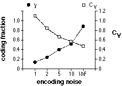
Figure 20. The stimulus s(t) and spike train x(t) were generated using the same model as illustrated for fig. 12. The Gaussian white noise r(t)was approximated by a discrete time step (0.5 ms) white Gaussian noise with variance sqrt(50 spk/s / 0.5 ms). The mean firing rate of the neuron model was 50 spk/s. See sect. 7.4 in chapter 9 of “Methods in Neuronal Modeling for the theoretical formulas).
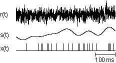
Figure 21 was obtained using the M-file sigmoid.m. Coherence values above the cut-off frequencies of 10 Hz were set to zero.
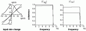
Figure 22 is a simple drawing.
